Analysis of in situ data with IPython
Some time ago I was responsible for a geotechnical report about a retaining wall in a lagoon. I only had a field of measures made up of: 6 CPTUs, 1 DTM and 3 soil samples. Hey a large amount of data! In that occasion I used a commercial software and a spreadsheet application, because the time was too little and I had not discovered IPython notebook yet. I show you through a short screencast how it is powerful and easy to use, perfect to this type of analysis.
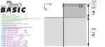
Anyway I could have used Octave (a Matlab clone) for doing the analysis, but probably I should have lost time for nothing. Let me show you the plan of investigations:
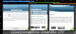
 |  |
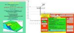
| Plan of investigations | Some diagrams from CPTU1 log (generated by IPython and Matplotlib) |
In spite of that, following a course available online by Coursera and called High Performance Scientific Computing, I could have examined first IPython and then its new rich text web interface: Notebook.
Citing the Official website, these are some features:
- Powerful interactive shells (terminal and Qt-based).
- A browser-based notebook with support for code, text, mathematical expressions, inline plots and other rich media.
- Support for interactive data visualization and use of GUI toolkits.
- Flexible, embeddable interpreters to load into your own projects.
- Easy to use, high performance tools for parallel computing.
All the same I don't want be bored with a long description, so I have created a screencast with a simple example where: I import a CPTU data and make a few plots. After the video, I put the instruction to install it in Ubuntu (or derivatives) and how to launch it. (09/06/2013) You can use it online instead, immediately without any set up but upon registration on Wakari (the Free Plan gives you 512 MB of ram and 10 GB of disk space). Let me just highlight two useful sites:
- loadtxt() function (some examples)
- Matplotlib tutorial by Nicolas P. Rougier.
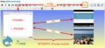
The screencast: load a cptu log and print diagrams using IPython notebook (NOTE: if that embedded media doesn't work, use this link).
Installation
First you have to install IPython and Matplot:
sudo apt-get install ipython
sudo apt-get install python-numpy
sudo apt-get install python-scipy
sudo apt-get install python-matplotlib
Finally up to date the last IPython version (the following commands will create a new directory named ipython):
git clone https://github.com/ipython/ipython.git
cd ipython
sudo python setup.py install
sudo python setup.py submodule
sudo python setup.py develop
Here it is the file I have created for diagrams (example_load_cptu_and_plot.ipynb):
{
 "metadata": {
  "name": "example_load_cptu_and_plot"
 },
 "nbformat": 3,
 "nbformat_minor": 0,
 "worksheets": [
  {
   "cells": [
    {
     "cell_type": "heading",
     "level": 1,
     "metadata": {},
     "source": [
      "A short example"
     ]
    },
    {
     "cell_type": "raw",
     "metadata": {},
     "source": [
      "Import data from a text file (cptu1_log.txt is in the same directory). Here it is some rows:\n",
      "# Depth (m)\tqc (MPa)\tfs (kPa)\tu (kPa)  (The first row is commented with '#')\n",
      "[...]\n",
      "2\t0.07\t0.5\t30.5\n",
      "2.02\t0.06\t1\t32.5\n",
      "2.04\t0.07\t0.5\t35.5\n",
      "2.06\t0.07\t0.5\t34\n",
      "2.08\t0.07\t0.5\t32.5\n",
      "2.1\t0.07\t0.5\t36.5\n",
      "[...]\n",
      "\n",
      "So I need 4 arrays for saving all the columns. Note: \"SHIFT + RETURN\" executes the code."
     ]
    },
    {
     "cell_type": "code",
     "collapsed": false,
     "input": [
      "depth, qc, fs, u = loadtxt(\"cptu1_log.txt\", usecols = (0,1,2,3), unpack=True)"
     ],
     "language": "python",
     "metadata": {},
     "outputs": []
    },
    {
     "cell_type": "raw",
     "metadata": {},
     "source": [
      "3 plot: -depth vs qc, -depth vs fs, -depth vs u"
     ]
    },
    {
     "cell_type": "code",
     "collapsed": false,
     "input": [
      "figure(figsize=(15,7.5), dpi=300)\n",
      "\n",
      "subplot(1,3,1)\n",
      "title('depth vs qc')\n",
      "ylabel('m')\n",
      "xlabel('MPa')\n",
      "plot (qc, -depth, color=\"red\",  linewidth=2.5, linestyle=\"-\")\n",
      "\n",
      "subplot(1,3,2)\n",
      "title('depth vs fs')\n",
      "ylabel('m')\n",
      "xlabel('kPa')\n",
      "plot (fs, -depth, color=\"black\",  linewidth=2.5, linestyle=\"-\")\n",
      "\n",
      "subplot(1,3,3)\n",
      "title('depth vs u')\n",
      "ylabel('m')\n",
      "xlabel('kPa')\n",
      "plot (u, -depth, color=\"blue\",  linewidth=2.5, linestyle=\"-\")"
     ],
     "language": "python",
     "metadata": {},
     "outputs": []
    }
   ],
   "metadata": {}
  }
 ]
}


Add new comment