About storm sewer design: an overview
In the past I created a little BASIC program to help me in the design of a storm sewer system, using the linear reservoir model. I am going to publish my work, but first I will introduce briefly the theory linked to this one. The article won't be too didactic and detailed, to do this I put some links.
The storm sewer is designed to drain excess rain and ground water from paved streets, parking lots, sidewalks, and roofs to collect them in proper deliveries.
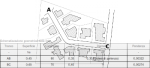
First the designer have to find the course of the system and the correct rainfall intensity-frequency-duration (IFD) curve (in Italy the return period is T=10 years for a small drained system). These are very difficult aspects to study, that include urbanization, topography, hydrology and statistic. Anyway for a little storm sewer system the path is along the streets and IFD curves are provided by local regulator.
To determine the flow and capacity due to the rainfall there are in literature many methods, like:
- rational method;
- linear reservoir model;
- Nash method.
I used to program my Sharp PC-E500 calculator, the linear reservoir model, but I don't scorn the others!
Linear reservoir model
Engineering acquires and applies mathematic, physic and natural knowledge, in order to design and build structures, machines, devices, systems, materials and processes. Linear reservoir model confirm this rule, because it reduces the unsteady flow with the uniform flow and the uni-dimensional continuity equation with the reservoir one.
Resulting equation can be adapted to open sections (rivers, drains, etc.) or to closed ones (pipes). The system course is divided into more little parts where they each receives rain flow for the interested surface. So that:
- each system part is characterized by a surface $S$, a length $L$ with a area section $A$ and a flow ratio $\phi$ (for example in a impermeable surface the flow ratio is $0.90$).
- in upstream of each one the continuity equation will be:
\[\begin{aligned}
p - Q & = {dV \over dt} & per \quad t \leq \tau \\
- Q & = {dV \over dt} & per \quad t > \tau
\end{aligned} \]
where:
$ \tau $ is duration of the rainfall;
$ V $ is the changed volume of the reservoir (in increasing or decreasing);
$ p $ is the flow that grows up in $dt$ time;
$ Q $ is the flow that goes out from each part.
 |  |
In the mathematical demonstration it is inserted in $p-Q = {dV \over dt}$ the relationship between the $Q$ flow and the $V$ volume:
$ V = V_0 {\bigl( {Q \over Q_0} \bigr)}^{1 \over \alpha}$ found from $Q= A v = c A^{\alpha}$ and $ {Q \over Q_0} = \bigl( {A \over A_0} \bigr)^{\alpha}$
The final equation will be:
$$ dt = { V_0 \over {\alpha Q_0^{1 \over \alpha}}} {{Q^{{1-\alpha} \over \alpha}} \over { p - Q }} dQ $$
In the pipes $\alpha = 1$ and for the storm sewers the main equations are:
\[\begin{aligned}
\epsilon &= 3.94 - 8.21 n + 6.23 n^2 \\
K_c &= \bigl( {{10 \phi a} \over {3.6^n \epsilon}} \bigr)^{1 \over {1-n}} {{1} \over {ln {\epsilon \over {\epsilon - 1}}}} \\
u &= \Bigl( {K_c \over {v_0}} \Bigr)^{{1 - n} \over {n}} \\
Q &= u S
\end{aligned} \]
Where:
- $a$ e $n$ are the IFD curve ratio: $ h = a \tau^n$, a is in $mm \cdot ore^{-n}$ because $\tau$ is expressed in hours, $n$ is dimensionless and always less than 1.
- $v_0$ is called reservoir volume and is the sum of $v_s$ (generally for Italy defined in $40 m^3/ha$), $v_c$ is the volume calculated for single part.
- $K_c$,$\epsilon$ e $u$ are assumptions taken during demonstration.
The preliminary modeling consists in the following choices:
- pipe type: shape section (every shape has a specific dimensionless table for the calculations) and material (for Gauckler-Strickler roughness coefficient);
- variable of reference for the calculus:
- gradient of the pipeline (on the plain is $0,2 \%$);
- speed limit between $0,5$ and $5$ m/s;
- shear stress $\tau$ (greater than 2 $N/m^2$).
The designing begin in the upstream of the system, where every part is calculated taking the rising up surface and yielding the commercial diameter. If the diameter between a part and the following one skips the expected size from the succession of commercial diameters (i.e. the first diameter is 200 and the second 300, jumping the intermediate commercial of 250 mm), then it is necessary subdivide the upstream line in two parts.
In a next article I will show you a little example for a small system. Then finally I publish my FreeBASIC code.
REFERENCES:
- For the hydraulic theory in this article I have used this book:
Luigi Da Deppo, Claudio Datei, Fognature, Padova, Cortina, 2002 - In Wikipedia there is a little introduction.
- More informations (in Italian) are collected in duplicated lecture noted written by lecturer Ignazio Mantica.


Add new comment